
The previous blog posts showed specific applications using the HEC-ResSim software. This post will show the creation of an HEC-ResSim model taking the reader through the Watershed Setup module, the Reservoir Network module, and the Simulation module.
The initial model development will be that of a flow through model. It is recommended that the initial model setup be a flow through model to test the connectivity of the stream network and the overall behavior of the initial model setup.
A flow through model consists of the following model characteristics:
1.) No rules of operation are entered into the model
2.) A constant inflow is applied at the upstream ends of the main stem and all tributaries
3.) The reservoirs are set to the top of the conservation pool and are releasing inflow in the lookback period.
4.) The routing is set to null routing.
Once the results of the flow through model verify the connectivity and behavior of the model, additional inflow points with correct inflows, updated rules of operation, updated lookback values, and updated routing information can be incorporated.
Step 1: Create a New Directory
For this example, I created a new folder on my local drive titled, "building a ResSim model".


Step 3: Draw Schematic in Watershed Setup
Stream alignments can be imported from a GIS shapefile, but for this example, the alignment will be drawn in. The stream is drawn first and then the reservoirs and computations points are added. Streams and reservoirs are drawn from upstream to downstream.
In this schematic, there is a main stream with a single reservoir. There are tributaries coming in to the main stream both upstream and downstream of the reservoir. I added the computation points named point 1 and point 2.

Step 4: Create and Save Configuration
Go to Watershed > Configuration Editor. The name given to the configuration is "sample build". The time step is 1 hour.

With the Watershed Setup completed, the Reservoir Network is then developed. In the Reservoir Network, the physical and operational data is input.
Step 5: Create the Reservoir and Dam Physical Data
Select the Reservoir Network module. Create a new network.

Right click on the reservoir and select Pool. Enter the elevation-storage data for the pool. Elevation-area data is needed for evaporation. It is left out of this example since we are ignoring evaporation for simplicity.


Step 11: Review Results
I first look at the flow into the reservoir (Junction CP1). This inflow should be 1,000 cfs since I have 500 cfs coming in at Junction 6 and Junction 7.

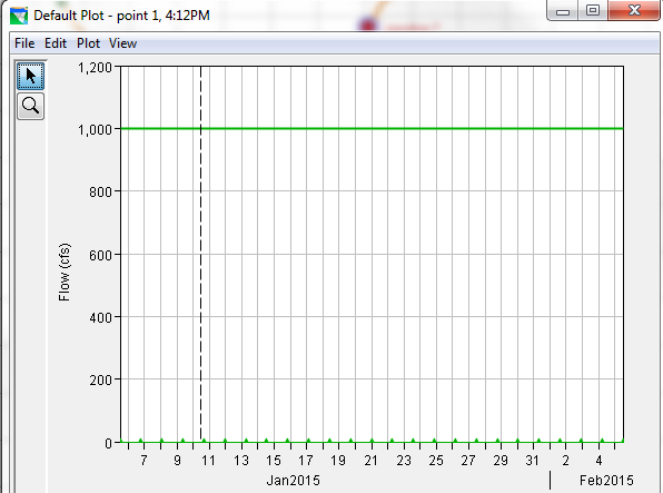
The junction, "Point 1", should have a flow a 1,000 cfs since that is being passed from the dam and there are no local inflows between the dam and "Point 1".

The junction, "Point 2", will have a local inflow of 500 cfs from the downstream tributary giving a total flow of 1,500 cfs when combined with the outflow from the dam.

At this point, we should feel comfortable that the model connectivity seems correct and that the behavior is what we would expect. New inflow locations, new operations sets with rules, and new routing parameters can be added.
To show a simple example, the flow through operation set will be duplicated and re-named max release. In this operation set, a maximum release rule of 750 cfs will be added.

The alternative named flow thru will be saved as "max rel". The operations set under the operations tab will be changed to max release.

Since the dates of our simulation are staying the same, we can add the max rel alternative to Jan-Feb 2015 sim and uncheck flow thru.


It is advisable to build ResSim models in this step by step method and to observe the results after each addition to the operational rules or changes to other parameters. It makes debugging the model much easier.
One final point is that this model was developed in English units. By selecting View > Unit System in the simulation module, the results can be viewed in SI.

The initial model development will be that of a flow through model. It is recommended that the initial model setup be a flow through model to test the connectivity of the stream network and the overall behavior of the initial model setup.
A flow through model consists of the following model characteristics:
1.) No rules of operation are entered into the model
2.) A constant inflow is applied at the upstream ends of the main stem and all tributaries
3.) The reservoirs are set to the top of the conservation pool and are releasing inflow in the lookback period.
4.) The routing is set to null routing.
Once the results of the flow through model verify the connectivity and behavior of the model, additional inflow points with correct inflows, updated rules of operation, updated lookback values, and updated routing information can be incorporated.
Step 1: Create a New Directory
For this example, I created a new folder on my local drive titled, "building a ResSim model".
Step 2: Create a New Model
Go to Tools > Options. Select the Model Directories tab. Select Add Location. Find the directory that you created in Step 1 and give the location a name. The name for this example is "Sample Build of ResSim model".

Go to File > New Watershed. Give the watershed a name and description. Select location name. Select units. Select time zone.

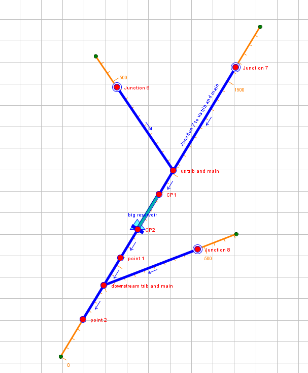
Stream alignments can be imported from a GIS shapefile, but for this example, the alignment will be drawn in. The stream is drawn first and then the reservoirs and computations points are added. Streams and reservoirs are drawn from upstream to downstream.
In this schematic, there is a main stream with a single reservoir. There are tributaries coming in to the main stream both upstream and downstream of the reservoir. I added the computation points named point 1 and point 2.

Step 4: Create and Save Configuration
Go to Watershed > Configuration Editor. The name given to the configuration is "sample build". The time step is 1 hour.

With the Watershed Setup completed, the Reservoir Network is then developed. In the Reservoir Network, the physical and operational data is input.
Step 5: Create the Reservoir and Dam Physical Data
Select the Reservoir Network module. Create a new network.


For this example, we will code one controlled outlet with a release capacity of 1,000 cfs for all elevations. Right click on Dam at main stream and select "Add controlled outlet".

Step 6: Create the Reservoir Operational Data
Go to Operations > New. Since we are developing a flow through model for testing, no rules are entered at this time, only the zone elevations. For this example, I put in elevations for top of flood control (75 ft), top of conservation (50 ft), and top of inactive (25 ft).

Step 7: Create the Routing Reaches
Before drawing the routing reaches, I recommend adding junctions to the confluence of the tributaries and the main stem. In the schematic below, I added the following junctions: "us trib and main" and "downstream trib and main". Note that junctions 6, 7, and 8 were added automatically when I created the reaches. Reaches are drawn from junction to junction upstream to downstream. The computation points, "point 1" and "point 2", become junctions in the Reservoir Network module. The default routing method of Null is used in the flow through model.
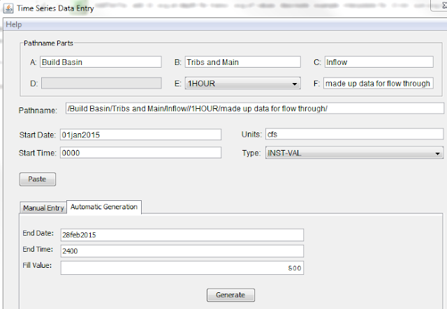
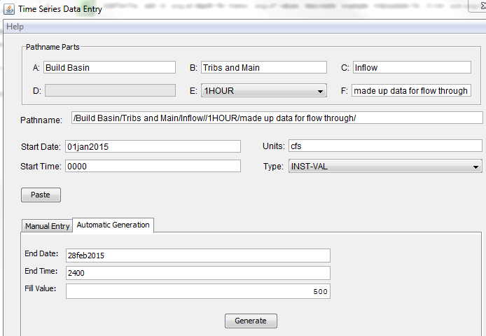
Step 8: Create the Inflow DSS File
For the flow through example, create a single dss file with a constant 500 cfs of inflow. This will be applied to the upstream end of the tributaries and the main stream.
Open HEC-DSSVue. Create a new DSS file in your shared sub-directory.

Under data entry, select "Manual Time Series". Enter the pathname parts with the time series increment. This data set is being created with a 1-hour increment. Use a start date and end date that will cover the entire simulation including lookback.
Step 9: Create Alternative
Go back to ResSim and create the alternative.
Set lookback elevation to top of conservation (50 ft) and the lookback release to the inflow (1000 cfs). These numbers will cause ResSim to hold top of conservation by releasing inflow. This will help test the proper functioning of the model before moving on to adding rules, routing parameters, etc.

Select flow through as your operations set.

Select upstream junctions in the model and indicate that inflow is coming in at these locations. The 1.0 factor means that the inflow from the DSS file will not be increased or decreased.

Select the DSS filename and path for the three inflow locations.


Finally, set time step to 1 hour under Run Control.
Step 10: Create and Run Simulation
Select Simulation > New. The lookback period is to ensure that model locations are populated with data once the simulation begins. You need to make sure that your lookback period and simulation period are covered by the data in your DSS file. Once this is complete, run your simulation.

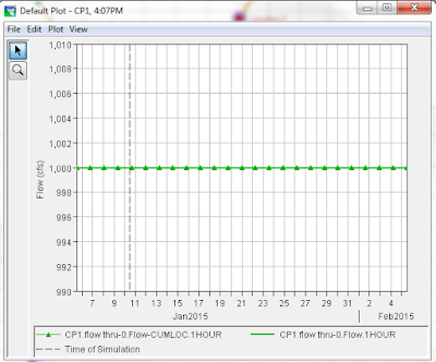
I first look at the flow into the reservoir (Junction CP1). This inflow should be 1,000 cfs since I have 500 cfs coming in at Junction 6 and Junction 7.

Since the dam has the capacity to pass the inflow and there are no rules of operation, I expect to see the pool elevation remain constant at top of conservation (50 ft) and the outflow to be 1,000 cfs.

The junction, "Point 1", should have a flow a 1,000 cfs since that is being passed from the dam and there are no local inflows between the dam and "Point 1".
The junction, "Point 2", will have a local inflow of 500 cfs from the downstream tributary giving a total flow of 1,500 cfs when combined with the outflow from the dam.

At this point, we should feel comfortable that the model connectivity seems correct and that the behavior is what we would expect. New inflow locations, new operations sets with rules, and new routing parameters can be added.
To show a simple example, the flow through operation set will be duplicated and re-named max release. In this operation set, a maximum release rule of 750 cfs will be added.

The alternative named flow thru will be saved as "max rel". The operations set under the operations tab will be changed to max release.

Since the dates of our simulation are staying the same, we can add the max rel alternative to Jan-Feb 2015 sim and uncheck flow thru.

Now, when the simulation is computed, there is a rise into the flood pool since the rule is limiting the maximum release below the inflow.

One final point is that this model was developed in English units. By selecting View > Unit System in the simulation module, the results can be viewed in SI.

No comments:
Post a Comment
Thanks for your comments