
Wednesday, 24 July 2019

Machine Learning Course in Python (Support Vector Machines)

Continuing on with the series, we will move on the support vector machines for programming assignment 6. If you had notice, I did not have a write-up for assignment 5 as most of the tasks just require plotting and interpretation of the learning curves. However, you can still find the code in my GitHub at https://github.com/Benlau93/Machine-Learning-by-Andrew-Ng-in-Python/tree/master/Bias_Vs_Variance.
There is two part in this assignment. First, we will implement Support Vector Machines (SVM) on several 2D data set to have an intuition of the algorithms and how it works. Next, we will use SVM on emails datasets to try and classify spam emails.
To load the dataset, loadmat from scipy.io is used to open the mat files
import numpy as np
import pandas as pd
import matplotlib.pyplot as plt
from scipy.io import loadmatmat = loadmat("ex6data1.mat")
X = mat["X"]
y = mat["y"]
Plotting of the dataset
m,n = X.shape[0],X.shape[1]
pos,neg= (y==1).reshape(m,1), (y==0).reshape(m,1)
plt.scatter(X[pos[:,0],0],X[pos[:,0],1],c="r",marker="+",s=50)
plt.scatter(X[neg[:,0],0],X[neg[:,0],1],c="y",marker="o",s=50)


We start off with a simple dataset that has a clear linear boundary between the training examples.
As recommended in the lecture, we try not to code SVM from scratch but instead, make use of highly optimized library such as sklearn for this assignment. The official documentation can be found here.
from sklearn.svm import SVC
classifier = SVC(kernel="linear")
classifier.fit(X,np.ravel(y))


Since this is a linear classification problem, we will not be using any kernel for this task. This is equivalent to using the linear kernel in SVC (note that the default kernel setting for SVC is “ rbf”, which stands for Radial basis function). The
ravel() function here returns an array with size (m, ) which is required for SVC.plt.figure(figsize=(8,6)) plt.scatter(X[pos[:,0],0],X[pos[:,0],1],c="r",marker="+",s=50) plt.scatter(X[neg[:,0],0],X[neg[:,0],1],c="y",marker="o",s=50)# plotting the decision boundary X_1,X_2 = np.meshgrid(np.linspace(X[:,0].min(),X[:,1].max(),num=100),np.linspace(X[:,1].min(),X[:,1].max(),num=100)) plt.contour(X_1,X_2,classifier.predict(np.array([X_1.ravel(),X_2.ravel()]).T).reshape(X_1.shape),1,colors="b") plt.xlim(0,4.5) plt.ylim(1.5,5)


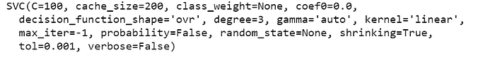
With the default setting of C = 1.0 (remember C = 1/λ), this is the decision boundary we obtained.
# Test C = 100
classifier2 = SVC(C=100,kernel="linear")
classifier2.fit(X,np.ravel(y))

plt.figure(figsize=(8,6))
plt.scatter(X[pos[:,0],0],X[pos[:,0],1],c="r",marker="+",s=50)
plt.scatter(X[neg[:,0],0],X[neg[:,0],1],c="y",marker="o",s=50)# plotting the decision boundary
X_3,X_4 = np.meshgrid(np.linspace(X[:,0].min(),X[:,1].max(),num=100),np.linspace(X[:,1].min(),X[:,1].max(),num=100))
plt.contour(X_3,X_4,classifier2.predict(np.array([X_3.ravel(),X_4.ravel()]).T).reshape(X_3.shape),1,colors="b")
plt.xlim(0,4.5)
plt.ylim(1.5,5)

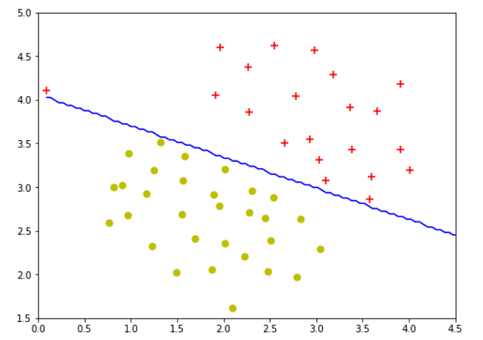
Changing C=100, gave a decision boundary that overfits the training examples.
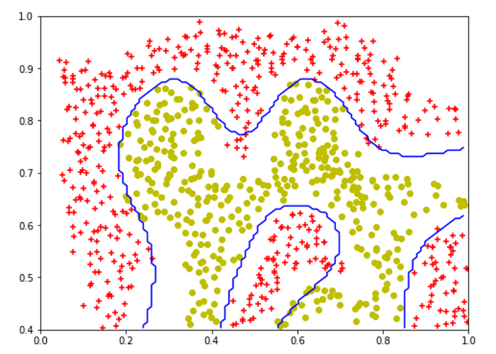
Next, we will look at a dataset that could not be linearly separable. Here is where kernels come into play to provide us with the functionality of a non-linear classifier. For those having difficulties comprehending the concept of kernels, this article I found gave a pretty good intuition and some mathematics explanation about kernels. For this part of the assignment, we were required to complete the function
gaussianKernel to aid in the implementation of SVM with Gaussian kernels. I will be skipping this step as SVC contain its own gaussian kernels implementation in the form of Radial basis function (rbf). Here is the Wikipedia page with the equation for rbf, as you can see, it is identical to the Gaussian kernel function from the course.
Loading and plotting of example dataset 2
mat2 = loadmat("ex6data2.mat")
X2 = mat2["X"]
y2 = mat2["y"]m2,n2 = X2.shape[0],X2.shape[1]
pos2,neg2= (y2==1).reshape(m2,1), (y2==0).reshape(m2,1)
plt.figure(figsize=(8,6))
plt.scatter(X2[pos2[:,0],0],X2[pos2[:,0],1],c="r",marker="+")
plt.scatter(X2[neg2[:,0],0],X2[neg2[:,0],1],c="y",marker="o")
plt.xlim(0,1)
plt.ylim(0.4,1)


To implement SVM with Gaussian kernels
classifier3 = SVC(kernel="rbf",gamma=30)
classifier3.fit(X2,y2.ravel())


In regards to the parameters of SVM with rbf kernel, it uses gamma instead of sigma. The documentation of the parameters can be found here. I found that gamma is similar to 1/σ but not exactly, I hope some domain expert can give me insights into the interpretation of this gamma term. As for this dataset, I found that gamma value of 30 shows the most resemblance to the optimized parameters in the assignment (sigma was 0.1 in the course).
plt.figure(figsize=(8,6))
plt.scatter(X2[pos2[:,0],0],X2[pos2[:,0],1],c="r",marker="+")
plt.scatter(X2[neg2[:,0],0],X2[neg2[:,0],1],c="y",marker="o")# plotting the decision boundary
X_5,X_6 = np.meshgrid(np.linspace(X2[:,0].min(),X2[:,1].max(),num=100),np.linspace(X2[:,1].min(),X2[:,1].max(),num=100))
plt.contour(X_5,X_6,classifier3.predict(np.array([X_5.ravel(),X_6.ravel()]).T).reshape(X_5.shape),1,colors="b")
plt.xlim(0,1)
plt.ylim(0.4,1)

As for the last dataset in this part, we perform a simple hyperparameter tuning to determine the best C and gamma values to use.
Loading and plotting of examples dataset 3
mat3 = loadmat("ex6data3.mat")
X3 = mat3["X"]
y3 = mat3["y"]
Xval = mat3["Xval"]
yval = mat3["yval"]m3,n3 = X3.shape[0],X3.shape[1]
pos3,neg3= (y3==1).reshape(m3,1), (y3==0).reshape(m3,1)
plt.figure(figsize=(8,6))
plt.scatter(X3[pos3[:,0],0],X3[pos3[:,0],1],c="r",marker="+",s=50)
plt.scatter(X3[neg3[:,0],0],X3[neg3[:,0],1],c="y",marker="o",s=50)


def dataset3Params(X, y, Xval, yval,vals):
    """
    Returns your choice of C and sigma. You should complete this function to return the optimal C and
    sigma based on a cross-validation set.
    """
    acc = 0
    best_c=0
    best_gamma=0
    for i in vals:
        C= i
        for j in vals:
            gamma = 1/j
            classifier = SVC(C=C,gamma=gamma)
            classifier.fit(X,y)
            prediction = classifier.predict(Xval)
            score = classifier.score(Xval,yval)
            if score>acc:
                acc =score
                best_c =C
                best_gamma=gamma
    return best_c, best_gamma
dataset3Params iterates through the list of vals given in the function and set C as vals and gamma as 1/vals. An SVC model is constructed using each combination of parameters and the accuracy of the validation set is computed. Based on the accuracy, the best model is chosen and the values for the respective C and gamma are returned.vals = [0.01, 0.03, 0.1, 0.3, 1, 3, 10, 30]
C, gamma = dataset3Params(X3, y3.ravel(), Xval, yval.ravel(),vals)
classifier4 = SVC(C=C,gamma=gamma)
classifier4.fit(X3,y3.ravel())


plt.figure(figsize=(8,6))
plt.scatter(X3[pos3[:,0],0],X3[pos3[:,0],1],c="r",marker="+",s=50)
plt.scatter(X3[neg3[:,0],0],X3[neg3[:,0],1],c="y",marker="o",s=50)# plotting the decision boundary
X_7,X_8 = np.meshgrid(np.linspace(X3[:,0].min(),X3[:,1].max(),num=100),np.linspace(X3[:,1].min(),X3[:,1].max(),num=100))
plt.contour(X_7,X_8,classifier4.predict(np.array([X_7.ravel(),X_8.ravel()]).T).reshape(X_7.shape),1,colors="b")
plt.xlim(-0.6,0.3)
plt.ylim(-0.7,0.5)

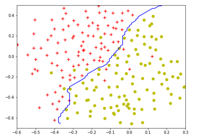
The optimal values are 0.3 for C and 100 for gamma, this results in similar decision boundary as the assginment.
Moving on to spam email classification. This problem is unique as it focuses more on data preprocessing than the actual modeling process. The emails need to process in a way that that could be used as input for the model. One way of doing so is to obtain the indices of all the words in an email based on a list of commonly used vocabulary.
Loading the data
import re
from nltk.stem import PorterStemmerfile_contents = open("emailSample1.txt","r").read()
vocabList = open("vocab.txt","r").read()


Vocabulary list and its respective indices were given, I had stored the list as a dictionary with the vocabs as keys and indices as values. You could probably do it another way but I want to make accessing the vocabs easier (eg. with
if keys in dict)vocabList=vocabList.split("\n")[:-1]vocabList_d={} for ea in vocabList: value,key = ea.split("\t")[:] vocabList_d[key] = value
As for preprocessing the emails, several steps were outlined for us in the assignment.
def processEmail(email_contents,vocabList_d):
    """
    Preprocesses the body of an email and returns a list of indices of the words contained in the email.
    """
    # Lower case
    email_contents = email_contents.lower()

    # Handle numbers
    email_contents = re.sub("[0-9]+","number",email_contents)

    # Handle URLS
    email_contents = re.sub("[http|https]://[^\s]*","httpaddr",email_contents)

    # Handle Email Addresses
    email_contents = re.sub("[^\s]+@[^\s]+","emailaddr",email_contents)

    # Handle $ sign
    email_contents = re.sub("[$]+","dollar",email_contents)

    # Strip all special characters
    specialChar = ["<","[","^",">","+","?","!","'",".",",",":"]
    for char in specialChar:
        email_contents = email_contents.replace(str(char),"")
    email_contents = email_contents.replace("\n"," ")

    # Stem the word
    ps = PorterStemmer()
    email_contents = [ps.stem(token) for token in email_contents.split(" ")]
    email_contents= " ".join(email_contents)

    # Process the email and return word_indices

    word_indices=[]

    for char in email_contents.split():
        if len(char) >1 and char in vocabList_d:
            word_indices.append(int(vocabList_d[char]))

    return word_indicesword_indices= processEmail(file_contents,vocabList_d)
The use of regular expression comes in very handy here, this tutorial by python guru can help you get started on re. The other useful library here is nlkt where the
PorterStemmer() function helps with stemming the words. Another good tutorial here, this time by pythonprogramming.net.
After getting the indices of the words, we need to convert the indices into a features vector.
def emailFeatures(word_indices, vocabList_d):
    """
    Takes in a word_indices vector and  produces a feature vector from the word indices.
    """
    n = len(vocabList_d)

    features = np.zeros((n,1))

    for i in word_indices:
        features[i] =1

    return featuresfeatures = emailFeatures(word_indices,vocabList_d)
print("Length of feature vector: ",len(features))
print("Number of non-zero entries: ",np.sum(features))
The print statement will print:
Length of feature vector: 1899 and Number of non-zero entries: 43.0 . This is slightly different from the assignment as you’re was captured as “you” and “re” in the assignment while my code identified it as “your”, resulting in lesser non-zero entries.
To train the SVM will be as simple as passing the features as input. However, this is only one training example and we will need more training data to train a classifier.
spam_mat = loadmat("spamTrain.mat")
X_train =spam_mat["X"]
y_train = spam_mat["y"]
Training examples are given in
spamTrain.mat to train our classifier while test examples are in spamTest.mat to determine our model generalizability.C =0.1
spam_svc = SVC(C=0.1,kernel ="linear")
spam_svc.fit(X_train,y_train.ravel())
print("Training Accuracy:",(spam_svc.score(X_train,y_train.ravel()))*100,"%")
The print statement will print:
Training Accuracy: 99.825 %spam_mat_test = loadmat("spamTest.mat") X_test = spam_mat_test["Xtest"] y_test =spam_mat_test["ytest"]spam_svc.predict(X_test) print("Test Accuracy:",(spam_svc.score(X_test,y_test.ravel()))*100,"%")
The print statement will print:
Test Accuracy: 98.9 %
To better understand our model, we could look at the weights of each word and figure out the words that are most predictive of a spam email.
weights = spam_svc.coef_[0]
weights_col = np.hstack((np.arange(1,1900).reshape(1899,1),weights.reshape(1899,1)))
df = pd.DataFrame(weights_col)df.sort_values(by=[1],ascending = False,inplace=True)predictors = []
idx=[]
for i in df[0][:15]:
    for keys, values in vocabList_d.items():
        if str(int(i)) == values:
            predictors.append(keys)
            idx.append(int(values))print("Top predictors of spam:")for _ in range(15):
    print(predictors[_],"\t\t",round(df[1][idx[_]-1],6))


That's it for support vector machines! The jupyter notebook will be uploaded to my GitHub at (https://github.com/Benlau93/Machine-Learning-by-Andrew-Ng-in-Python).
Wednesday, 17 July 2019
MongoDB Tutorial
MongoDB is an open-source document database and leading NoSQL database. MongoDB is written in C++. This tutorial will give you great understanding on MongoDB concepts needed to create and deploy a highly scalable and performance-oriented database.
Audience
This tutorial is designed for Software Professionals who are willing to learn MongoDB Database in simple and easy steps. It will throw light on MongoDB concepts and after completing this tutorial you will be at an intermediate level of expertise, from where you can take yourself at higher level of expertise.
Prerequisites
Before proceeding with this tutorial, you should have a basic understanding of database, text editor and execution of programs, etc. Because we are going to develop high performance database, so it will be good if you have an understanding on the basic concepts of Database (RDBMS).
xxxxxxxxxxxxxxxxxxxxxxxx
MongoDB is a cross-platform, document oriented database that provides, high performance, high availability, and easy scalability. MongoDB works on concept of collection and document.
Database
Database is a physical container for collections. Each database gets its own set of files on the file system. A single MongoDB server typically has multiple databases.
Collection
Collection is a group of MongoDB documents. It is the equivalent of an RDBMS table. A collection exists within a single database. Collections do not enforce a schema. Documents within a collection can have different fields. Typically, all documents in a collection are of similar or related purpose.
Document
A document is a set of key-value pairs. Documents have dynamic schema. Dynamic schema means that documents in the same collection do not need to have the same set of fields or structure, and common fields in a collection's documents may hold different types of data.
The following table shows the relationship of RDBMS terminology with MongoDB.
| RDBMS | MongoDB |
|---|---|
| Database | Database |
| Table | Collection |
| Tuple/Row | Document |
| column | Field |
| Table Join | Embedded Documents |
| Primary Key | Primary Key (Default key _id provided by mongodb itself) |
| Database Server and Client | |
| Mysqld/Oracle | mongod |
| mysql/sqlplus | mongo |
Sample Document
Following example shows the document structure of a blog site, which is simply a comma separated key value pair.
{
   _id: ObjectId(7df78ad8902c)
   title: 'MongoDB Overview',
   description: 'MongoDB is no sql database',
   by: 'tutorials point',
   url: 'http://www.tutorialspoint.com',
   tags: ['mongodb', 'database', 'NoSQL'],
   likes: 100,
   comments: [
      {
         user:'user1',
         message: 'My first comment',
         dateCreated: new Date(2011,1,20,2,15),
         like: 0
      },
      {
         user:'user2',
         message: 'My second comments',
         dateCreated: new Date(2011,1,25,7,45),
         like: 5
      }
   ]
}
_id is a 12 bytes hexadecimal number which assures the uniqueness of every document. You can provide _id while inserting the document. If you don’t provide then MongoDB provides a unique id for every document. These 12 bytes first 4 bytes for the current timestamp, next 3 bytes for machine id, next 2 bytes for process id of MongoDB server and remaining 3 bytes are simple incremental VALUE.
xxxxxxxxxxxxxxxxxxxxxx
Any relational database has a typical schema design that shows number of tables and the relationship between these tables. While in MongoDB, there is no concept of relationship.
Advantages of MongoDB over RDBMS
- Schema less − MongoDB is a document database in which one collection holds different documents. Number of fields, content and size of the document can differ from one document to another.
- Structure of a single object is clear.
- No complex joins.
- Deep query-ability. MongoDB supports dynamic queries on documents using a document-based query language that's nearly as powerful as SQL.
- Tuning.
- Ease of scale-out − MongoDB is easy to scale.
- Conversion/mapping of application objects to database objects not needed.
- Uses internal memory for storing the (windowed) working set, enabling faster access of data.
Why Use MongoDB?
- Document Oriented Storage − Data is stored in the form of JSON style documents.
- Index on any attribute
- Replication and high availability
- Auto-sharding
- Rich queries
- Fast in-place updates
- Professional support by MongoDB
Where to Use MongoDB?
- Big Data
- Content Management and Delivery
- Mobile and Social Infrastructure
- User Data Management
- Data Hub
xxxxxxxxxxxxxxxxxxxxxx
Let us now see how to install MongoDB on Windows.
Install MongoDB On Windows
To install MongoDB on Windows, first download the latest release of MongoDB from https://www.mongodb.org/downloads. Make sure you get correct version of MongoDB depending upon your Windows version. To get your Windows version, open command prompt and execute the following command.
C:\>wmic os get osarchitecture
OSArchitecture
64-bit
C:\>
32-bit versions of MongoDB only support databases smaller than 2GB and suitable only for testing and evaluation purposes.
Now extract your downloaded file to c:\ drive or any other location. Make sure the name of the extracted folder is mongodb-win32-i386-[version] or mongodb-win32-x86_64-[version]. Here [version] is the version of MongoDB download.
Next, open the command prompt and run the following command.
C:\>move mongodb-win64-* mongodb
   1 dir(s) moved.
C:\>
In case you have extracted the MongoDB at different location, then go to that path by using command cd FOOLDER/DIR and now run the above given process.
MongoDB requires a data folder to store its files. The default location for the MongoDB data directory is c:\data\db. So you need to create this folder using the Command Prompt. Execute the following command sequence.
C:\>md data
C:\md data\db
If you have to install the MongoDB at a different location, then you need to specify an alternate path for \data\db by setting the path dbpath in mongod.exe. For the same, issue the following commands.
In the command prompt, navigate to the bin directory present in the MongoDB installation folder. Suppose my installation folder is D:\set up\mongodb
C:\Users\XYZ>d:
D:\>cd "set up"
D:\set up>cd mongodb
D:\set up\mongodb>cd bin
D:\set up\mongodb\bin>mongod.exe --dbpath "d:\set up\mongodb\data"
This will show waiting for connections message on the console output, which indicates that the mongod.exe process is running successfully.
Now to run the MongoDB, you need to open another command prompt and issue the following command.
D:\set up\mongodb\bin>mongo.exe
MongoDB shell version: 2.4.6
connecting to: test
>db.test.save( { a: 1 } )
>db.test.find()
{ "_id" : ObjectId(5879b0f65a56a454), "a" : 1 }
>
This will show that MongoDB is installed and run successfully. Next time when you run MongoDB, you need to issue only commands.
D:\set up\mongodb\bin>mongod.exe --dbpath "d:\set up\mongodb\data"
D:\set up\mongodb\bin>mongo.exe
Install MongoDB on Ubuntu
Run the following command to import the MongoDB public GPG key −
sudo apt-key adv --keyserver hkp://keyserver.ubuntu.com:80 --recv 7F0CEB10
Create a /etc/apt/sources.list.d/mongodb.list file using the following command.
echo 'deb http://downloads-distro.mongodb.org/repo/ubuntu-upstart dist 10gen'
   | sudo tee /etc/apt/sources.list.d/mongodb.list
Now issue the following command to update the repository −
sudo apt-get update
Next install the MongoDB by using the following command −
apt-get install mongodb-10gen = 2.2.3
In the above installation, 2.2.3 is currently released MongoDB version. Make sure to install the latest version always. Now MongoDB is installed successfully.
Start MongoDB
sudo service mongodb start
Stop MongoDB
sudo service mongodb stop
Restart MongoDB
sudo service mongodb restart
To use MongoDB run the following command.
mongo
This will connect you to running MongoDB instance.
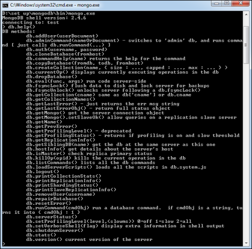
MongoDB Help
To get a list of commands, type db.help() in MongoDB client. This will give you a list of commands as shown in the following screenshot.
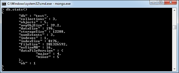
MongoDB Statistics
To get stats about MongoDB server, type the command db.stats() in MongoDB client. This will show the database name, number of collection and documents in the database. Output of the command is shown in the following screenshot.
xxxxxxxxxxxxxxxxxxxxxxxxxData in MongoDB has a flexible schema.documents in the same collection. They do not need to have the same set of fields or structure, and common fields in a collection’s documents may hold different types of data.
Some considerations while designing Schema in MongoDB
- Design your schema according to user requirements.
- Combine objects into one document if you will use them together. Otherwise separate them (but make sure there should not be need of joins).
- Duplicate the data (but limited) because disk space is cheap as compare to compute time.
- Do joins while write, not on read.
- Optimize your schema for most frequent use cases.
- Do complex aggregation in the schema.
Example
Suppose a client needs a database design for his blog/website and see the differences between RDBMS and MongoDB schema design. Website has the following requirements.
- Every post has the unique title, description and url.
- Every post can have one or more tags.
- Every post has the name of its publisher and total number of likes.
- Every post has comments given by users along with their name, message, data-time and likes.
- On each post, there can be zero or more comments.
In RDBMS schema, design for above requirements will have minimum three tables.

While in MongoDB schema, design will have one collection post and the following structure −
{
   _id: POST_ID
   title: TITLE_OF_POST,
   description: POST_DESCRIPTION,
   by: POST_BY,
   url: URL_OF_POST,
   tags: [TAG1, TAG2, TAG3],
   likes: TOTAL_LIKES,
   comments: [
      {
         user:'COMMENT_BY',
         message: TEXT,
         dateCreated: DATE_TIME,
         like: LIKES
      },
      {
         user:'COMMENT_BY',
         message: TEXT,
         dateCreated: DATE_TIME,
         like: LIKES
      }
   ]
}
So while showing the data, in RDBMS you need to join three tables and in MongoDB, data will be shown from one collection only.
Subscribe to:
Posts (Atom)